Excel: Heat maps

A heat map is a great place to get an overall view of the data.

• Applying color using conditional formatting

Excel allows you apply color to values in spreadsheet using the ‘Conditional Formqatting’ tool.

1. Select the area of the heat map required.

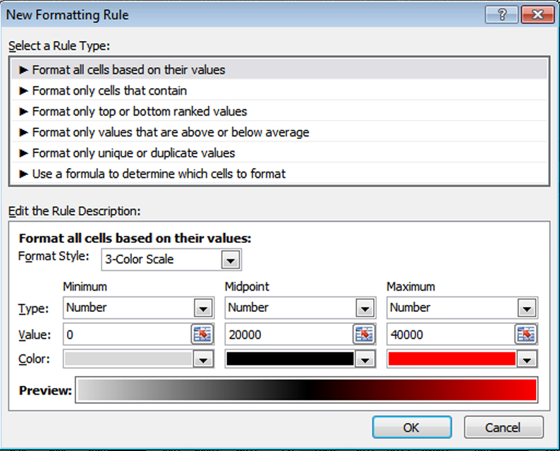
2. Click ‘Conditional Formatting’ from the top menu bar and select ‘New Rule’. Edit the rule description to your liking. Your rules might look something like this:

• Exporting to Powerpoint

The simplest method is to select the area you want from the Excel spreadsheet, copy, and paste into powerpoint. Use ‘Paste Special’ to paste as a ‘Picture (Enhanced Metafile)’ to preserve the conditional formatting.

Here is a trick for making the numbers disappear from a heat map in Excel:

1. Select the area of the heat map required.

2. Find the ‘Format Cells’ panel – either click on the bottom right hand corner of the ‘Number’ box or the Format button in the ‘Cells’ box and select ‘Format Cells’.

3. In the Format Cells panel, select ‘Custom’ from the list in the ‘Category:’ panel and select ;;; from the ‘Type:’ menu (or type ;;; in the box over where it says “General”). Click OK.